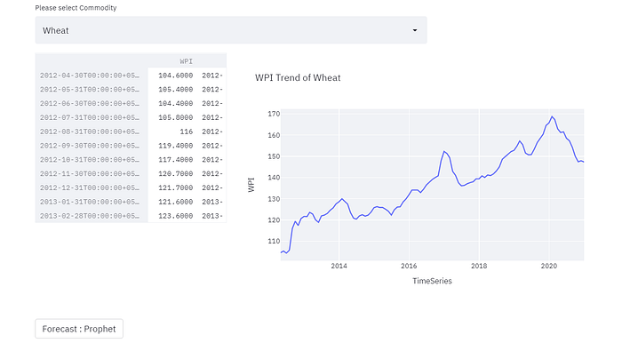
By applying the Time Series forecasting we can able to forecast the inflation rate of particular good. A data source can be downloaded from https://eaindustry.nic.in/. The dataset contains different commodities data. We can select any required goods we are interested in forecasting.
We are going to build a forecasting model using Prophet and integrate it with Streamlit. Source Code available at https://github.com/raouday79/wpi-forecasting
Data preprocessing: let's view the data in our data frame.

Filter the data on the selected commodity. Drop the first two rows. Time is in columns needs to change into rows. Python provides the melt function for this.
#Dropping the Column
comm1.drop([‘COMM_CODE’,’COMM_WT’],inplace=True, axis = 1)
comm1.head(5)reshaped_df = comm1.melt(id_vars=[‘COMM_NAME’],var_name=’Month-Year’,value_name=’WPI’)
reshaped_df.head(10)reshaped_df[‘Month-Year’] = reshaped_df[‘Month-Year’].str.replace(‘INDX’, ‘’)
reshaped_df.head(2)
reshaped_df.tail(2)
Generate the Time Series using the pandas date_range function
time_series = pd.date_range(start=’04/30/2012', end=’12/31/2020', freq=’M’)
duration = pd.DataFrame(data={“TimeSeries”:time_series},index=time_series)reshaped_df[‘TimeSeries’] = duration.index
Time Series will help in imputing the missing value if any for the month. After that, you can join the two data frames.
Exploratory Data Analysis: let's perform the box plot for the outlier detection in the dataset. we can use seaborn’s boxflot.

We can check the normal distribution of the data Histogram Plot.

We have data as monthly granularity. we can plot to check the seasonality trend and level by seasonal decomposition.
from statsmodels.tsa.seasonal import seasonal_decompose
from matplotlib.dates import DateFormatter
from matplotlib import dates as mpld
product_data = reshaped_df
result_add = seasonal_decompose(product_data[‘WPI’],model=’additive’,period=12)
result_add.plot()
plt.gcf().autofmt_xdate()
date_format = mpld.DateFormatter(‘%y-%m’)
plt.gca().xaxis.set_major_formatter(date_format)
We can visualize the trend is increasing and seasonality exist in selected commodity.
Building Model: Let's split the data into training and testing. As we are using the time-series data. The split will be on the time horizon.
model_building_df = product_data
model_building_df[‘TimeSeries’] = model_building_df.index
#Model building
# Choose prediction step
prediction_size = 2 #Test Data Size
train_dataset= pd.DataFrame()
train_dataset[‘ds’] = pd.to_datetime(model_building_df[‘TimeSeries’])
train_dataset[‘y’]=model_building_df[targetVariable]
#train_dataset[‘AvgtempC’] = product_data[‘AvgtempC’]
#train_dataset[‘PrecipMM’] = product_data[‘PrecipMM’]train_df = train_dataset.iloc[:len(train_dataset)-prediction_size,:]
test_df = train_dataset.iloc[len(train_dataset)-prediction_size:,:]pro_regressor= Prophet(growth=’linear’,daily_seasonality=False,weekly_seasonality=False,yearly_seasonality=False,
seasonality_mode=’multiplicative’,
changepoint_prior_scale=0.05,
)
#pro_regressor.add_country_holidays(country_name=’IN’)
#pro_regressor.add_regressor(‘AvgtempC’)
#pro_regressor.add_regressor(‘PrecipMM’)
pro_regressor.fit(train_df)
future_data = pro_regressor.make_future_dataframe(periods=prediction_size,freq=’M’)# — — — — — — — — — — Chooose Frequency
#future_data[‘AvgtempC’]=train_dataset[‘AvgtempC’]
#future_data[‘PrecipMM’]=train_dataset[‘PrecipMM’]
#future_data[‘AvgtempC’] = future_data[‘AvgtempC’].replace(np.nan,25)
#future_data[‘PrecipMM’] = future_data[‘PrecipMM’].replace(np.nan,0)
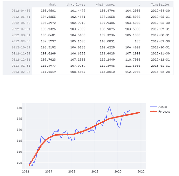
forecast_data = pro_regressor.predict(test_df)
fig = pro_regressor.plot(forecast_data);forecaste = pro_regressor.predict(future_data)
fig = pro_regressor.plot(forecaste);
a = add_changepoints_to_plot(fig.gca(), pro_regressor, forecaste)


Making Future Forecast:


We can integrate the forecasting model with Streamlit for creating the Web App.
We can forecast the inflation of any commodity. The full source available at https://github.com/raouday79/wpi-forecasting
Thank You.
Keep Learning..Keep Exploring.